
Predicting diabetes and ENT emergency department admissions using hospital records
Introduction
Healthcare costs are increasing at a rapid and unsustainable rate. According to the Centers for Medicare and Medicaid Services, in 2018, national health expenditures increased by 4.6% to $11,172 per person (1). One area that seems promising to reduce healthcare costs, for both hospitals and individuals, is to reduce avoidable admissions to the emergency department (ED). Between 2008 and 2012, visits to the ED without admission to the hospital increased by 11.4% (2). If many of these ED visits that do not lead to hospital admissions are for minor reasons, they could be seen as preventable. Although some situations require the use of the ED, others can be handled at urgent care facilities. Still, others can be completely avoided through preventative care. Identifying the patients that are likely to visit the ED when they do not need to do so could save hospital systems both time and money. Logistic regression is a common technique to identify high-risk patients, but more recently, machine learning models have been used in prediction. In this paper, we evaluate how well five different types of predictive models perform at identifying patients most likely to visit the ED. Additionally, we include multiple novel predictors in our models to improve prediction, including familial tendency to visit the ED and patient distance to the ED, and we identify which features may be most useful when predicting ED visits.
One class of diseases that can often be treated through preventative care or at an urgent care facility is an Ambulatory Care Sensitive Condition (ACSC). Billings et al. (3) define these conditions as “diagnoses for which timely and effective outpatient care can help to reduce the risks of hospitalization by either preventing the onset of an illness or condition, controlling an acute episodic illness or condition, or managing a chronic disease or condition”. Among these diseases are chronic conditions, such as diabetes, and more acute illnesses, such as ear, nose, and throat (ENT) conditions. We examine two separate cohorts with an ACSC. The first cohort includes patients 18 years old or older who have diabetes. These patients should be working with their primary care physician to take preventative measures to avoid a visit to the ED. Thus, a visit to the ED due to diabetes for these patients may be considered an avoidable admission. The second cohort includes all children under the age of 18. For this cohort, we are interested in whether a patient has an ED visit due to an ENT condition. Among these conditions are tonsillitis, pharyngitis, and respiratory infections. Preventative care or visiting an urgent care facility can keep these patients out of the ED, so a visit to the ED for an ENT condition may also be considered an avoidable admission. We choose to focus on diabetes and ENT conditions since, for the healthcare system we consider here, they account for the largest proportion of ED visits for an ACSC for chronic conditions in adults and acute conditions in children, respectively.
Since many ED visits due to diabetes or ENT conditions are avoidable, a healthcare system could likely reduce both their own costs and the costs incurred by their patients by conducting a targeted outreach program to patients most at risk of avoidable ED visits. Targeted outreach programs have had success in other areas, such as in prenatal care (4). To conduct a targeted outreach program for avoidable ED visits, a healthcare system would need to know which patients are most at risk of visiting the ED. Past researchers have identified a variety of different factors that lead to an elevated risk of an ED visit or hospital admission, including a person’s socioeconomic status, race, and medical history (3,5-9). These researchers have typically used logistic regression, but more recently, machine learning methods have been used to identify high risk patients, including the lasso, random forests, gradient boosting, and decision trees (10-17). However, there is very little known about the relative performance of these different models in the setting of identifying high-risk patients, something we examine in this paper. Another aspect of avoidable admissions that has not been fully considered is how a patient’s location may affect their risk of an ED visit for an ACSC, though some researchers have incorporated some spatial information in their models (3,13,16,18). However, the impact of spatial variables on avoidable ED admissions for our two cohorts is largely unknown and has not been coupled with the set of variables we employ in this article. Finally, we consider how a patient’s familial tendencies to visit the ED may impact the patient’s risk of going to the ED.
In the following section, we discuss the different statistical models we use to predict ED visits. We then present our results and provide a brief discussion of our findings.
Methods
Our data set consists of patients in the state of Utah insured by a single insurance provider. The study was conducted in accordance with the Declaration of Helsinki (as revised in 2013). The study was approved by the Intermountain Healthcare Privacy Board (#1051166) and informed consent was deemed not necessary. We selected all members of this insurer who were either an adult diagnosed with diabetes (for the diabetes model) or a child (for the ENT model). The response variable in our model is whether a patient visits the ED in each quarter due to either an ENT condition or diabetes. The explanatory variables used to predict whether a patient visits the ED in a given quarter are based on information gathered on the final day of the previous quarter.
The first columns in Table 1 and Table 2 list the explanatory variables used for the diabetes and ENT cohorts, respectively. These variables can be grouped into the following descriptive classes: (I) demographic; (II) socioeconomic [based on the census block (CB) in which a person lives, including the Singh area deprivation index (ADI), a composite index representing the socioeconomic status of a region]; (III) medical history (including diabetes type for the diabetes model, inferred by the time since first diagnosis—patients that received their first diagnosis when 20 years old or younger were assumed to have Type I diabetes); (IV) geographic; and (V) temporal.
Table 1
| Variable | Training set | Test set |
|---|---|---|
| Number of patients | 43,999 | 31,740 |
| Number of quarters | 310,546 | 31,740 |
| Number of emergency department visits | 1,968 | 178 |
| Ethnicity | ||
| Not Hispanic* | 38,716 (0.88) | 27,905 (0.88) |
| Hispanic | 4,713 (0.11) | 3,473 (0.11) |
| Unknown | 570 (0.01) | 362 (0.01) |
| Marital status | ||
| Married | 28,134 (0.64) | 20,341 (0.64) |
| Single* | 8,034 (0.18) | 5,564 (0.18) |
| Divorced | 4,806 (0.11) | 3,450 (0.11) |
| Widowed | 2,296 (0.05) | 1,856 (0.06) |
| Separated | 510 (0.01) | 349 (0.01) |
| Unknown | 219 (0) | 180 (0.01) |
| Race | ||
| White* | 40,405 (0.92) | 29,257 (0.92) |
| Unknown | 1,077 (0.02) | 718 (0.02) |
| Asian | 807 (0.02) | 631 (0.02) |
| Native Hawaiian or Pacific Islander | 759 (0.02) | 482 (0.02) |
| Black | 490 (0.01) | 339 (0.01) |
| American Indian or Alaska Native | 461 (0.01) | 313 (0.01) |
| Religiosity | ||
| Religious* | 33,133 (0.75) | 29,162 (0.92) |
| Not available | 9,126 (0.21) | 1,859 (0.06) |
| Not religious | 1,740 (0.04) | 719 (0.02) |
| Sex | ||
| Female* | 23,541 (0.54) | 17,070 (0.54) |
| Male | 20,458 (0.46) | 14,670 (0.46) |
| Location | ||
| Urban | 41,315 (0.94) | 29,806 (0.94) |
| Rural* | 2,684 (0.06) | 1,934 (0.06) |
| Diabetes complications | ||
| Has no complications* | 35,009 (0.8) | 22,771 (0.72) |
| Has complications | 8,990 (0.2) | 8,969 (0.28) |
| Diabetes type | ||
| Type II* | 41,184 (0.94) | 29,770 (0.94) |
| Type I | 2,815 (0.06) | 1,970 (0.06) |
| Primary care physician | ||
| Designated | 41,200 (0.94) | 30,324 (0.96) |
| Not designated* | 2,799 (0.06) | 1,416 (0.04) |
| Age (years) | 55.93 (15.13) | 56.11 (15.19) |
| Proportion occupied by owner | 0.72 (0.22) | 0.72 (0.22) |
| Proportion single parent with dependents | 0.09 (0.05) | 0.09 (0.05) |
| Median family income | 68,068 (24,928.77) | 68,283.21 (24,979.15) |
| Median home value | 221,318.7 (90,792.66) | 221,920.64 (91,362.2) |
| Median monthly mortgage | 1,471.29 (425.64) | 1,474.63 (425.25) |
| Proportion below 1.5 times the poverty level | 0.22 (0.15) | 0.22 (0.15) |
| Proportion below poverty level | 0.1 (0.1) | 0.1 (0.1) |
| Proportion with high school education | 0.9 (0.09) | 0.91 (0.09) |
| Singh area deprivation index | 100.16 (16.9) | 100.03 (16.99) |
| Proportion unemployed | 0.08 (0.05) | 0.08 (0.05) |
| Number of behavioral conditions | 0.63 (1.1) | 0.6 (1.04) |
| Number of Charlson comorbidities | 2.88 (1.87) | 2.94 (1.89) |
| Number of days since first diagnosis | 3,088.24 (2,136.56) | 3,346.23 (2,218.41) |
| Past emergency department visits/quarter for other reasons | 0.02 (0.11) | 0.02 (0.07) |
| Past emergency department visits/quarter by family for other reasons | 0.01 (0.05) | 0.01 (0.04) |
| Past emergency department visits/quarter by family for diabetes | 0 (0.02) | 0 (0.02) |
| Past emergency department visits/quarter for diabetes/ear, nose, and throat conditions | 0.01 (0.07) | 0.01 (0.05) |
| Weight | 96.86 (26.73) | 97.01 (26.8) |
| Drive time to emergency department | 13.22 (14.07) | 12.96 (13.52) |
| Difference in drive time to emergency department over urgent care | 3.82 (17.65) | 3.6 (17.28) |
*, denotes reference level when modeling. The data are shown as means or proportions.
Table 2
| Variable | Training set | Test set |
|---|---|---|
| Number of patients | 361,430 | 225,414 |
| Number of quarters | 2,435,319 | 225,414 |
| Number of emergency department visits | 7890 | 730 |
| Ethnicity | ||
| Not Hispanic* | 254,880 (0.71) | 164,277 (0.73) |
| Unknown | 61,440 (0.17) | 32,449 (0.14) |
| Hispanic | 45,110 (0.12) | 28,688 (0.13) |
| Race | ||
| White* | 293,904 (0.81) | 187,527 (0.83) |
| Unknown | 49724 (0.14) | 26,849 (0.12) |
| Native Hawaiian or Pacific Islander | 5,677 (0.02) | 3,356 (0.01) |
| Black | 4,949 (0.01) | 3,118 (0.01) |
| Asian | 4,711 (0.01) | 3,108 (0.01) |
| American Indian or Alaska Native | 1,973 (0.01) | 1,173 (0.01) |
| Multiple | 492 (0) | 283 (0) |
| Religiosity | ||
| Religious* | 236,208 (0.65) | 170,861 (0.76) |
| Not available | 94,816 (0.26) | 37,442 (0.17) |
| Not religious | 30,406 (0.08) | 17,111 (0.08) |
| Sex | ||
| Male | 185,745 (0.51) | 115,890 (0.51) |
| Female* | 175,685 (0.49) | 109,524 (0.49) |
| Location | ||
| Urban | 341,058 (0.94) | 212,507 (0.94) |
| Rural* | 20,372 (0.06) | 12,907 (0.06) |
| Primary care physician | ||
| Designated | 325,203 (0.9) | 210,400 (0.93) |
| Not designated* | 36,227 (0.1) | 15,014 (0.07) |
| Age (years) | 8.4 (5.08) | 9.14 (4.73) |
| Proportion occupied by owner | 0.74 (0.21) | 0.75 (0.21) |
| Proportion single parent with dependents | 0.09 (0.04) | 0.09 (0.04) |
| Median family income | 70,937.53 (25,233.6) | 71,138.07 (25,040.81) |
| Median home value | 232,059.35 (95157.83) | 232,475.48 (94,767.7) |
| Median monthly mortgage | 1,527.66 (434.32) | 1,530.65 (431.05) |
| Proportion below 1.5 times the poverty level | 0.2 (0.15) | 0.2 (0.15) |
| Proportion below poverty level | 0.09 (0.1) | 0.09 (0.1) |
| Proportion with high school education | 0.92 (0.09) | 0.92 (0.08) |
| Singh area deprivation index | 98.06 (17.59) | 97.96 (17.49) |
| Proportion unemployed | 0.07 (0.05) | 0.07 (0.05) |
| Number of behavioral conditions | 0.11 (0.47) | 0.12 (0.49) |
| Number of Charlson comorbidities | 0.14 (0.38) | 0.15 (0.39) |
| Past emergency department visits/quarter for other reasons | 0 (0.04) | 0 (0.03) |
| Past emergency department visits/quarter by family for other reasons | 0.01 (0.06) | 0.01 (0.04) |
| Past emergency department visits/quarter by family for ear, nose, and throat conditions | 0 (0.02) | 0 (0.01) |
| Past emergency department visits/quarter for diabetes/ear, nose, and throat conditions | 0 (0.04) | 0 (0.02) |
| Drive time to emergency department | 13.46 (14.91) | 13.39 (14.57) |
| Difference in drive time to emergency department over urgent care | 4.48 (16.86) | 4.32 (16.82) |
*, denotes reference level when modeling. The data are shown as means or proportions.
We split the data into a training set and a test set. The training set includes 10 total quarters, spanning from the third quarter of 2016 to the last quarter of 2018. The test set includes patient outcomes for the first quarter of 2019. Using this training and test set, we select the final predictive models for identifying patients at risk of an ED visit for diabetes or an ENT condition.
Tables 1,2 show basic summary information for the patients in each cohort, including counts and proportions for the categorical variables and means and standard deviations for the numeric variables. The diabetes cohort overall is a majority White, non-Hispanic, married, religious, and urban. Most of the patients have Type II diabetes, no past complications, and a primary care physician. The ENT cohort overall is also a majority White, non-Hispanic, religious, and urban.
Statistical analysis
To predict which patients are at risk of visiting the ED for both ACSCs of interest, we fit five predictive classification models. Due to the large number of possible explanatory variables in the data set, we use a lasso within logistic regression to aid in variable selection. We also employ a mixed effects logistic regression model (using the covariates chosen from the lasso) with a random effect for the patient’s small geographic area, a random forest model, and a gradient boosted model using XGBoost. Finally, to have a baseline for comparison, we fit a naive logistic regression model with only one predictor: the number of past visits to the ED per quarter.
Logistic regression with a lasso uses a penalization parameter to shrink the size of the variables’ coefficients toward zero, where variables are removed from the model if their coefficient shrinks to zero exactly, making it a useful technique for variable selection. Variables that are collinear or not useful in prediction are often eliminated so the most important variables remain in the model.
For the mixed effects model, we use the same covariates chosen using the lasso model. The utility of the mixed model is that it can include random effects for other variables, adjusting for the fact that some of the data may be correlated (19). In this case, we include a random effect for the small geographic area where a person lives, as there may be some correlation in the probability of an ED visit for people who live in the same area. For example, a certain area may have more spread of ENT conditions, resulting in people who live in that area being more likely to visit the ED than people who live in other areas.
The first machine learning technique we consider is a random forest model. To understand a random forest model (and the XGBoost model described below), it is first important to understand decision trees. A decision tree starts with every observation in the same group, or classification (for example, at risk or not at risk). That group is then split into two groups by some variable that best distinguishes observations with similar responses. Then, one of those two branches is split into two more branches so that the new branches have observations with the most similar responses. The branch and variable are chosen so that the groups in each branch are most uniform. The tree continues to be divided until none of the branches can be divided further (given limitations, such as each end branch containing a minimum number of patients or the tree reaching a maximum number of splits). When predicting the probability that a given patient goes to the ED, we simply calculate the proportion of patients that went to the ED in the final branch where the patient ends up given their characteristics.
A single decision tree is subject to a high degree of variability. If we were to add more patients to the data set, it could drastically change the way the model decides to split the tree. A random forest model (20), which fits hundreds of trees, is much more stable. Creating multiple trees with the same data and the same variables would lead to repeatedly creating the exact same tree, so to end up with many distinct trees (or a forest), for each tree, the algorithm uses a sample of the data, and for each branch, the algorithm only includes a fraction of the variables when deciding how to split the tree. After fitting hundreds of trees, when predicting whether a patient will go to the ED, the algorithm makes a prediction using each tree. It then combines all predictions into a single probability that the patient will go to the ED.
The other machine learning technique we use to predict ED admissions is XGBoost, short for Extreme Gradient Boosting (21). Gradient boosting is like random forest in that we make many decision trees, but the nature of the trees is different. In XGBoost, after making a single decision tree, we calculate the residuals for that tree. We then use the residuals from that tree to build a second tree, add the predicted residuals to the original prediction, and recalculate the residuals. Since building trees based on residuals could quickly lead to overfitting the training data, before adding the residuals to the original prediction, we scale down the residuals by some learning rate parameter. Additionally, the predicted residuals include a regularization parameter to help prevent overfitting. The process of building a tree to predict residuals, adding the residuals to the prediction, and recalculating the residuals continues for a specified number of trees, or until model improvement stagnates.
The last model we fit is a naive logistic regression model using only the patient’s past visits to the ED per quarter for either diabetes or an ENT condition to predict future visits. If the only thing useful in predicting a patient’s future ED visits is their past visits, the other models will struggle to outperform this simple model. There is value in using a simple, easy to explain model, so if this model performs just as well as the others, it would be easier to explain the results and implement the model.
To evaluate model performance, we use precision-recall curves. A precision-recall curve shows the proportion of patients who were predicted to visit the ED who actually did (precision) against the proportion of patients who visited the ED who were predicted to do so (recall). In other words, precision is the accuracy of the people we identified as going to the ED, while recall is the true positive rate. Ideally, a model should have both high precision and high recall, meaning the people who we identified as going to the ED were likely to go and the people who were likely to go to the ED were identified. A high precision with a low recall signifies that a model is accurate when it predicts a visit to the ED but that it does not predict many visits to the ED, so it is not a very useful model. A low precision with a high recall signifies a model that predicts many people going to the ED, encompassing most of the people that actually went to the ED, but also many of the people that did not. Finding the balance between the two is important because a targeted outreach campaign needs to reach enough people that it can make an impact, but not so many that it would be too costly to run.
Results
Figure 1 shows the precision-recall curves for each model predicting which patients will end up in the ED for a diabetes-related cause. The curves begin when recall is at least 2% and stop when 25% of patients are predicted to go to the ED. The five models perform similarly, though for most levels of recall, the XGBoost model gives the greatest precision. The other four models outperform the naive model at lower levels of recall. This indicates that people with the highest risk of going to the ED have other risk factors apart from previous ED visits. Once we start identifying patients with less risk, the naive model is competitive with the others, and it performs the best when recall is roughly between 25% and 37%.
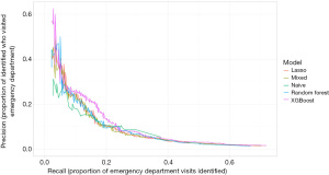
The C-index for the diabetes XGBoost model in the validation set (out of sample) is 0.80. In the training set (in sample) the C-index is 0.93. Both values show that our model and data are sufficiently predictive.
Tables 3,4 present the information for specific cases. Assuming a hospital system contacted the patients with the highest 0.5% or 2% of risk from the five models, these tables show the precision, recall, number of total patients who would be contacted, and the number of those contacted patients who went to the ED (or ED visits that could potentially be prevented). If a hospital system conducted a small, targeted outreach program and contacted the 0.5% of diabetes patients most at risk according to our models (about 150 patients), and helped those patients avoid going to the ED, they could possibly prevent up to 17% of the ED visits due to diabetes. If they conducted a larger outreach program and contacted the patients with the top 2% of risk, they could potentially prevent up to about 30% of diabetes ED visits from the cohort. Undoubtedly, such a program would not successfully eliminate every ED visit from someone contacted, but it has the potential to do a lot of good.
Table 3
| Model | Recall | Precision | Contacted | Prevented |
|---|---|---|---|---|
| Lasso | 0.152 | 0.172 | 157 | 27 |
| Mixed | 0.135 | 0.152 | 158 | 24 |
| Naive | 0.129 | 0.154 | 149 | 23 |
| Random forest | 0.146 | 0.165 | 158 | 26 |
| XGBoost | 0.169 | 0.190 | 158 | 30 |
Table 4
| Model | Recall | Precision | Contacted | Prevented |
|---|---|---|---|---|
| Lasso | 0.253 | 0.071 | 633 | 45 |
| Mixed | 0.258 | 0.073 | 632 | 46 |
| Naive | 0.298 | 0.086 | 615 | 53 |
| Random forest | 0.275 | 0.077 | 634 | 49 |
| XGBoost | 0.287 | 0.081 | 633 | 51 |
The precision-recall curves for the models predicting ED visits for ENT causes are shown in Figure 2. Again, the XGBoost model has the highest precision for most levels of recall. The C-index for the ENT XGBoost model in the validation set (out of sample) is 0.80. In the training set (in sample) the C-index is 0.86. Additionally, Tables 5,6 show the precision, recall, number of patients contacted, and number of potential ED visits prevented if a healthcare company conducted a targeted outreach program to 0.5% or 2.5% of the patients in the ENT cohort who had the highest probability of going to the ED according to our models. Note that because this cohort is noticeably larger than the diabetes cohort, the program would need to contact many more people, though it could also have a greater impact. If the hospital system conducted a small, targeted outreach program and reached out to the families of patients with the highest 0.5% of risk of going to the ED for an ENT condition (about 1,100 families), they could potentially prevent up to 11.8% of the ED visits (up to about 86 visits). If they conducted a slightly larger program and reached out to the families of patients with the highest 2.5% of risk (about 5,600 families), they could potentially prevent up to about 25.8% of ED visits for ENT conditions.
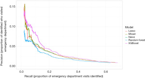
Table 5
| Model | Recall | Precision | Contacted | Prevented |
|---|---|---|---|---|
| Lasso | 0.089 | 0.058 | 1,124 | 65 |
| Mixed | 0.090 | 0.059 | 1,121 | 66 |
| Naive | 0.088 | 0.062 | 1,035 | 64 |
| Random forest | 0.086 | 0.056 | 1,125 | 63 |
| XGBoost | 0.118 | 0.077 | 1,122 | 86 |
Table 6
| Model | Recall | Precision | Contacted | Prevented |
|---|---|---|---|---|
| Lasso | 0.236 | 0.031 | 5,613 | 172 |
| Mixed | 0.240 | 0.031 | 5,585 | 175 |
| Naive | 0.238 | 0.031 | 5,628 | 174 |
| Random forest | 0.207 | 0.027 | 5,623 | 151 |
| XGBoost | 0.258 | 0.033 | 5,623 | 188 |
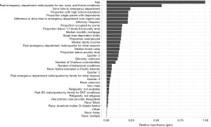
Since the XGBoost model generally has the best precision-recall curves for both cohorts, we first examine these models in more detail. As XGBoost is a tree-based technique, we cannot directly extract interpretable coefficients from the models; however, we can examine variable importance plots to understand which variables are most effective at making splits in the decision trees. The variable importance plots for the diabetes model and ENT model are shown in Figure 3 and Figure 4, respectively.
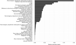
In the diabetes model, the most important variables in predicting whether someone will visit the ED are the patient’s past visits to the ED due to diabetes, the number of days since the patient’s first diabetes diagnosis (possibly indicating long-term diabetes patients), age, and weight. This does not necessarily mean there is a linear relationship between these variables and the probability of an ED visit, but that there is some information contained in these variables that is useful. The drive time for the patient to the ED is the next most important variable, while the difference in drive time to the ED and urgent care is also relatively important, indicating geography does impact a patient’s risk of going to the ED. The demographic variables, such as sex, marital status, ethnicity, race, and religiosity, have the lowest relative importance.
In the ENT model, age and the number of past visits per quarter for an ENT condition are the most important predictors of visiting the ED. Drive time to the ED and difference in drive time to the ED and urgent care are also important variables. The demographic variables again have the lowest relative importance.
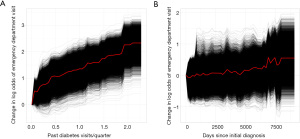
One way to understand the effects of the most important variables in the XGBoost models is through examining partial dependence plots. Figure 5A shows the effect of the past number of ED visits per quarter, while holding other variable effects constant, on the log odds of someone going to the ED for diabetes. The black lines represent how changing the explanatory variable affects the log odds of individual patients in the cohort, while the red line is the average across all patients. Figure 5B shows the effect of the number of days since the patient’s initial diabetes diagnosis. These plots make it clear that having many past visits to the ED for diabetes dramatically increases a patient’s risk of going to the ED, while having had diabetes for longer may slightly increase a patient’s risk.
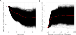
The variable importance plot for the ENT cohort indicates that age and the number of past ED visits for ENT conditions are the most important factors in the probability of a patient going to the ED for an ENT condition. Figure 6A contains a partial dependence plot for the effect of age, while Figure 6B contains a partial dependence plot for the effect of past visits to the ED for ENT conditions. Overall, younger patients are much more likely to go to the ED for an ENT condition, while having any past visits to the ED for an ENT condition increases a patient’s risk.
Although the other models are generally outperformed by the XGBoost models, some insights can be gained by looking at the results from the lasso and mixed models. These models have interpretable coefficients which can be used to identify why someone might have a higher risk of visiting the ED. A positive coefficient signifies a factor that leads to increased risk, while a negative coefficient signifies a factor that leads to decreased risk. The estimated log odds ratios and their 95% confidence intervals that are statistically significant at the α=0.05 level are shown in Figure 7.
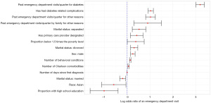
When interpreting the effects of the covariates in our model, it is important to acknowledge that the size and direction of each effect reflects holding all other variable effects constant. Of the demographic variables, having the marital status of separated or divorced (as compared to single) increases risk of going to the ED for diabetes, while having a marital status of married decreases the risk. According to the model, males are also significantly more likely to visit the ED for diabetes than females, and Asians are less likely to go to the ED than White people. Of the socioeconomic variables, having a higher proportion of the CB below the 1.5 times the poverty line is associated with more ED visits, while having more of the CB with a high school education leads to decreased risk.
Of the medical history variables, people with more past visits for diabetes per quarter are more likely to go to the ED for diabetes in the future. Additionally, people with more past visits to the ED for other reasons are also more likely to visit the ED for diabetes in the future. Having family members with many past visits to the ED for other reasons also leads to elevated risk of going to the ED for diabetes for the patient. Having diabetes with complications, rather than without past complications, also leads to a higher risk of future ED visits. According to this model, patients with a primary care physician designated are more likely to visit the ED. This could reflect those patients at high-risk may be more likely to have a primary care physician designated. Patients with a larger number of behavioral health conditions and Charlson comorbidities are more likely to visit the ED. Finally, patients who have had diabetes for longer (largely patients with type I diabetes) are more likely to visit the ED.
The geographic variables are not significant at the 0.05 level, though the drive time to the ED variable is somewhat compelling (P=0.087). The XGBoost model has drive time to the ED as one of its most important variables, but the mixed model did not identify this as a strong effect.
Figure 8 shows the estimated log odds ratios and their 95% confidence intervals of the statistically significant variables at the α=0.05 level from the ENT mixed model. Those of Hispanic ethnicity are significantly more likely to visit the ED with an ENT condition when compared to people with a non-Hispanic ethnicity. Children with race listed as Black, American Indian/Alaska Native, or Native Hawaiian/Pacific Islander have more risk of going to the ED (compared to White children). Finally, children from families that identified as not religious have less risk compared to children who are from families that identified as religious.
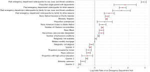
There are some socioeconomic variables that are useful in predicting future ED admissions. Children that live in CBs with a higher median monthly mortgage, a higher proportion of homes occupied by the owner, and a higher proportion of people with a high school education are significantly less likely to visit the ED, while children that live in CBs with a high proportion of single parents with dependents and a higher proportion of people unemployed are significantly more likely to visit the ED for an ENT condition. The geographic variables are not strong predictors of whether a child will go to the ED for an ENT condition in the mixed model. This is a contrast to the XGBoost model, where both drive time to the ED and difference and drive time to the ED and urgent care are important variables.
As with the diabetes model, children with a primary care physician designated are more likely to go to the ED for an ENT condition. Having more behavioral conditions, more Charlson comorbidities, or more ED visits in the past (either for ENT conditions or any other condition) leads to elevated risk of a future ED visit for an ENT condition. Past family visits to the ED (either for ENT conditions or any other condition) are also related to future ED visits for ENT conditions. Finally, children are significantly more likely to visit the ED for an ENT condition in the first quarter of the year (January–March), which makes sense, as the first quarter largely coincides with winter.
Discussion
Although the XGBoost model slightly outperformed the other models, the lasso and mixed models (and even the naive model using only past visits to the ED) had comparable precision-recall curves. For some levels of recall in the diabetes model, the naive model did the best. Though there is room for more advanced machine learning methods in predicting avoidable ED admissions, more basic statistical methods are still useful. Of the methods we used, the XGBoost model performed the best overall, similar to what was found by Rahimian et al. (15), though surprisingly, random forest was our weakest predicting method. Others, including Panicacci et al. (14), have had more success with random forests.
When deciding which model to use in a targeted outreach program, there are multiple factors that need to be considered. One factor is the size of such a program. In the diabetes case, the other models outperformed the naive model at identifying high-risk patients, but the naive model did just as well, if not better, at identifying patients that still had moderate risk of going to the ED. Thus, for a larger program, the naive model might be a better choice than the more complex models. A second factor to consider is how well each model performs in prediction. Generally, the XGBoost model performed the best, especially in the ENT case, indicating that there may be some complex interactions or nonlinear effects in someone’s risk of visiting the ED. If a hospital system wants the best identification of high-risk patients possible and is willing to use a less interpretable model than the others, we would recommend using our XGBoost model. However, the final factor that needs to be considered is the ease of using the model in a targeted outreach program. Because such a program may be expensive to run, it needs buy-in from decision makers, who may not be as comfortable using machine learning models. Even among the regression-type models, there is a difference in the ease of implementation. The naive logistic regression model only requires one input, a patient’s past visits to the ED, making it easier to explain and possibly easier to implement with competitive results. Additionally, implementation of such a program could be easier, as the hospital system would only need to reach out to patients that have past visits to the ED and explain that past visits is a large risk factor of future visits. The lasso and mixed models serve as a compromise between the XGBoost and naive models, giving some interpretability, but better prediction than the naive model at lower levels of recall. Our random forest model performs poorly in prediction and is not as easy to explain, so we would not recommend using it in this case.
For the ENT cohort, we recommend that a targeted outreach program be created based on the predictions from the XGBoost model, regardless of the size of the program. Although the model is less interpretable than the others, it does much better at prediction. If there is a need for a regression-type model, the naive logistic regression model compares favorably to the lasso and mixed models. Again, our random forest model performs poorly relative to the other models in prediction and should not be used in this case.
Past visits to the ED for diabetes, ENT conditions, or unrelated conditions are strong predictors of whether someone will visit the ED in future quarters. The number of past visits to the ED by family members is also a good predictor of whether someone will go to the ED for diabetes or an ENT condition. This was an interesting result from our models, as it was one of the features that we identified few other models using. Future models predicting ED visits should incorporate familial tendencies of ED visits when possible. Other medical history information, including the number of Charlson comorbidities and the number of behavioral conditions of the patient, are strong predictors of an ED admission. For both cohorts, patients with an assigned primary care physician are more likely to visit the ED, which seems somewhat counterintuitive. We could speculate that patients with higher risk may be more likely to have a primary care physician, but the nature of this relationship is unclear.
Some socioeconomic indicators are useful in predicting ED admissions. In both models, having a high proportion of the CB with at least a high school education is associated with fewer ED visits, meaning more educated areas might have a lower risk of going to the ED. In the ENT model, children who live in CBs with a high proportion of single parents with dependents and a higher proportion of people unemployed are significantly more likely to visit the ED, meaning children who live in poorer areas or with a single parent may be more likely to end up in the ED. This supports the finding from Billings et al. (3) that people who live in lower-income areas are more likely to be admitted to the hospital for an ACSC, though they also found that this effect was not as large for children or elderly people, while we have identified the effect for children with ENT conditions.
Geography plays some role in the probability that a person visits the ED. In the diabetes XGBoost model, a patient’s distance to the ED is the fifth most important variable, while in the ENT XGBoost model, it is the third most important variable. That effect seems larger in the XGBoost model than the other models, as the effect of drive time to the ED was non-significant in both mixed models. The mixed model slightly outperformed the lasso model in prediction, so incorporating a random effect for a patient’s small geographic area was useful. Overall, there may be some utility in using distance to the ED or a patient’s small geographic area in future models, but it is less essential than other important variables.
Overall, these models and variables are useful in identifying patients that may be at risk of going to the ED for either diabetes or an ENT condition. With enough resources, a targeted outreach program that relies on these models to identify at-risk patients could decrease the number of visits to the ED, saving resources for the hospital system and patients alike.
Acknowledgments
Mark Nielsen was instrumental in formulating the problem, creating the data set, and advising in modeling. Andy Merrill, Sean Miner, Joseph Sears, and Sage Roney helped formulate the problem and create and organize the data set used for modeling.
Funding: None.
Footnote
Data Sharing Statement: Available at https://jhmhp.amegroups.com/article/view/10.21037/jhmhp-22-3/dss
Conflicts of Interest: All authors have completed the ICMJE uniform disclosure form (available at https://jhmhp.amegroups.com/article/view/10.21037/jhmhp-22-3/coif). The authors have no conflicts of interest to declare.
Ethical Statement: The authors are accountable for all aspects of the work in ensuring that questions related to the accuracy or integrity of any part of the work are appropriately investigated and resolved. The study was conducted in accordance with the Declaration of Helsinki (as revised in 2013). The study was approved by the Intermountain Healthcare Privacy Board (#1051166) and informed consent was deemed not necessary.
Open Access Statement: This is an Open Access article distributed in accordance with the Creative Commons Attribution-NonCommercial-NoDerivs 4.0 International License (CC BY-NC-ND 4.0), which permits the non-commercial replication and distribution of the article with the strict proviso that no changes or edits are made and the original work is properly cited (including links to both the formal publication through the relevant DOI and the license). See: https://creativecommons.org/licenses/by-nc-nd/4.0/.
References
- CMS. NHE fact sheet (2018). Available online: https://www.cms.gov/Research-Statistics-Data-and-Systems/Statistics-Trends-and-Reports/NationalHealthExpendData/NHE-Fact-Sheet#:~:text=Historical%20NHE%2C%202020%3A,16%20percent%20of%20total%20NHE
- Fingar KR, Barrett ML, Elixhauser A, et al. Trends in potentially preventable inpatient hospital admissions and emergency department visits: Statistical brief #195 2016.
- Billings J, Zeitel L, Lukomnik J, et al. Impact of socioeconomic status on hospital use in New York City. Health Aff (Millwood) 1993;12:162-73. [Crossref] [PubMed]
- Maddox W. Avoiding pre-term birth with text messages in Dallas. D Magazine 2019. Available online: https://www.dmagazine.com/healthcare-business/2019/08/avoiding-pre-term-birth-with-text-messages-in-dallas/
- Kalinich M, Murphy W, Wongvibulsin S, et al. Prediction of severe immune-related adverse events requiring hospital admission in patients on immune checkpoint inhibitors: study of a population level insurance claims database from the USA. J Immunother Cancer 2021;9:e001935. [Crossref] [PubMed]
- Maleki MR, Doosty F, Yarmohammadian MH, et al. Designing an Elderly Hospital Admission Risk Prediction Model in Iran's Hospitals. Int J Prev Med 2021;12:22. [Crossref] [PubMed]
- Booth GL, Hux JE. Relationship between avoidable hospitalizations for diabetes mellitus and income level. Arch Intern Med 2003;163:101-6. [Crossref] [PubMed]
- Karunakaran A, Zhao H, Rubin DJ. Pre-and post-discharge risk factors for hospital readmission among patients with diabetes. Med Care 2018;56:634. [Crossref] [PubMed]
- Pappas G, Hadden WC, Kozak LJ, et al. Potentially avoidable hospitalizations: inequalities in rates between US socioeconomic groups. Am J Public Health 1997;87:811-6. [Crossref] [PubMed]
- Chen S, Bergman D, Miller K, et al. Using applied machine learning to predict healthcare utilization based on socioeconomic determinants of care. Am J Manag Care 2020;26:26-31. [Crossref] [PubMed]
- Corey KM, Kashyap S, Lorenzi E, et al. Development and validation of machine learning models to identify high-risk surgical patients using automatically curated electronic health record data (Pythia): A retrospective, single-site study. PLoS Med 2018;15:e1002701. [Crossref] [PubMed]
- Donnan PT, Dorward DW, Mutch B, et al. Development and validation of a model for predicting emergency admissions over the next year (PEONY): a UK historical cohort study. Arch Intern Med 2008;168:1416-22. [Crossref] [PubMed]
- Gao J, Moran E, Li YF, et al. Predicting potentially avoidable hospitalizations. Med Care 2014;52:164-71. [Crossref] [PubMed]
- Panicacci S, Donati M, Fanucci L, et al. Population health management exploiting machine learning algorithms to identify high-risk patients, in 2018 IEEE 31st International Symposium on Computer-Based Medical Systems (CBMS). IEEE 2018:298-303.
- Rahimian F, Salimi-Khorshidi G, Payberah AH, et al. Predicting the risk of emergency admission with machine learning: Development and validation using linked electronic health records. PLoS Med 2018;15:e1002695. [Crossref] [PubMed]
- Shadmi E, Flaks-Manov N, Hoshen M, et al. Predicting 30-day readmissions with preadmission electronic health record data. Med Care 2015;53:283-9. [Crossref] [PubMed]
- De Hond A, Raven W, Schinkelshoek L, et al. Machine learning for developing a prediction model of hospital admission of emergency department patients: Hype or hope? Int J Med Inform 2021;152:104496. [Crossref] [PubMed]
- Wan H, Zhang L, Witz S, et al. A literature review of preventable hospital readmissions: preceding the readmissions reduction act. IISE Trans Healthc Sys t Eng 2016;6:193-211.
- Gilmour A, Anderson R, Rae A. The analysis of binomial data by a generalized linear mixed model. Biometrika 1985;72:593-9.
- Breiman L. Random forests. Machine learning 2001;45:5-32. [Crossref] [PubMed]
- Chen T and Guestrin C. XGBoost: A scalable tree boosting system. In Proceedings of the 22nd ACM SIGKDD International Conference on Knowledge Discovery and Data Mining 2016:785-94.
Cite this article as: Ott A, Zabriskie BN, Hartman B. Predicting diabetes and ENT emergency department admissions using hospital records. J Hosp Manag Health Policy 2022;6:34.

